First tutorial: Getting started
In the first tutorial we’ll look at the basic components of epyc, and how to define and
run experiments on a single machine.
Note
The code for this tutorial can be found in the Github repository.
Concepts
epyc is built around three core concepts: experiments, labs, and notebooks.
An experiment is just an object inheriting from the Experiment class. An experiment can contain
pretty much any code you like, which is then called according to a strict protocol (described in detail
in The lifecycle of an experiment). The most important thing about experiments is that they can be parameterised with a set
of parameters passed to your code as a dict.
Parameters can come directly from calling code if the experiment is called directly, but it is more common for
experiments to be invoked from a lab. A lab defines a parameter space, a collection of parameters whose values
are each taken from a range. The set of all possible combinations of parameter values forms a multi-dimensional space,
and the lab runs an experiment for each point in that space (each combination of values). This allows the same
experiment to be done across a whole range of parameters with a single command. Different lab implementations provide
simple local sequential execution of experiments, parallel execution on a multicore machine, or parallel and
distributed execution on a compute cluster or in the cloud. The same experiment can usually be performed in any
lab, with epyc taking care of all the house-keeping needed. This makes it easy to scale-out experiments
over larger parameter spaces or numbers of repetitions.
Running the experiment produces results, which are stored in result sets collected
together to form a notebook. Result sets collect together the results from multiple
experimental runs. Each result contains the parameters of the experiment, the results
obtained, and some metadata describing how the experimental run proceeded. A result
set is hoogeneous, in the sense that the names of parameters, results, and metata will be the
same for all the results in the result set (although the values will of course be different).
Results can be searched and retrieved either as Python dicts or as pandas dataframes.
However, result sets are immutable: once results have been entered, they can’t be modified
or discarded.
By contrast, notebooks are heterogeneous, containing result sets with different experiments and sets of parameters and results. Notebooks can also be persistent, for example storing their results in JSON or HDF5 for easy access from other tools.
A repeatable computational environment
Before we dive in, we should adopt best practices and make sure that we have a controlled computational environment in which to perform experiments. See Reproducing experiments reliably for a thorough discussion of these topics.
A simple experiment
Computational experiments that justify using infrastructure like epyc are by definition
usually large and complicated – and not suitable for a tutorial. So we’ll start with a
very simple example: admittedly you could do this more easily with straight Python code,
but that’s an advantage when describing how to use a more complicated set-up.
So suppose we want to compute a set of values for some function so that we can plot
them as a graph. A complex function, or one that involved simulation, might justify
using epyc. For the time being let’s use a simple function:
We’ll plot this function about \((0, 0)\) extending \(2 \pi\) radians in each axial direction.
Defining the experiment
We first create a class describing our experiment. We do this by extending
Experiment and overriding Experiment.do() to provide the code actually executed:
from epyc import Experiment, Lab, JSONLabNotebook
import numpy

class CurveExperiment(Experiment):

    def do(self, params):
        '''Compute the sin value from two parameters x and y, returning a dict
        containing a result key with the computed value.

        :param params: the parameters
        :returns: the result dict'''
        x = params['x']
        y = params['y']
        r = numpy.sin(numpy.sqrt(x**2 + y**2))
        return dict(result = r)
That’s it: the code for the computational experiment, that will be executed at a point driven by the provided parameters dict.
Types of results from the experiment
epyc tries to be very Pythonic as regards the types one can return
from experiments. However, a lot of scientific computing must
interoperate with other tools, which makes some Python types less than
attractive.
The following Python types are safe to use in epyc result sets:
intfloatcomplexstringbool- one-dimensional arrays of the above
- empty arrays
There are some elements of experimental metadata that use exceptions or datestamps: these get special handling.
Also note that epyc can handle lists and one-dimensional arrays in
notebooks, but it can’t handle higher-dimensional arrays. If you
have a matrix, for example, it needs to be unpacked into one or more
one-dimensional vectors. This is unfortunate in general but not often
an issue in practice.
There are some conversions that happen when results are saved to
persistent notebooks, using either JSON (JSONLabNotebook) or
HDF5 (HDF5LabNotebook): see the class documentation for the
details (or if unexpected things happen), but generally it’s fairly
transparent when you stick top the types listed above.
Testing the experiment
Good development practice demands that we now test the experiment before running it in anger.
Usually this would involve writing unit tests within a framework provided by Python’s unittest
library, but that’s beyond the scope of this tutorial: we’ll simply run the experiment at a point
for which we know the answer:
# set up the test
params = dict()
params['x'] = 0
params['y'] = 0
res = numpy.sin(numpy.sqrt(x**2 + y**2))   # so we know the answer

# run the experiment
e = CurveExperiment()
rc = e.set(params).run()
print(rc[epyc.RESULTS]['result'] == res)
The result should be True. Don’t worry about how we’ve accessed the result: that’ll become
clear in a minute.
A lab for the experiment
To perform our experiment properly, we need to run the experiment at a lot of points,
to give use a “point cloud” dataset that we can then plot to see the shape of the function.
epyc lets us define the space of parameters over which we want to run the experiment,
and then will automatically run and collect results.
The object that controls this process is a Lab, which we’ll create first:
lab = Lab()
This is the most basic use of labs, which will store the results in an in-memory LabNotebook.
For more serious use, if we wanted to save the results for later, then we can create an persistent
JSONLabNotebook that stores results in a file in a JSON encoding:
lab = Lab(notebook = JSONLabNotebook("sin.json",
create = True,
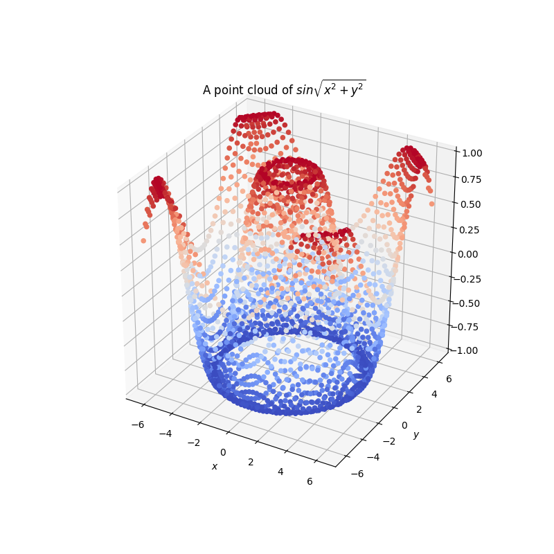
description = "A point cloud of $sin \sqrt{x^2 + y^2}$"))
This creates a JSON file with the name given in the first argument. The create argument, if set to True,
will overwrite the contents of the file; it defaults to False, which will load the contents of the file
instead, allowing the notebook to be extended with further results. The description is just free text.
Important
epyc lab notebooks are always immutable: you can delete them, but you can’t change their contents
(at least not from within epyc). This is intended to avoid the loss of data.
Specifying the experimental parameters
We next need to specify the parameter space over which we want the lab to run the experiment. This is done by mapping variables to values in a dict. The keys of the dict match the parameter values references in the experiment; the values can be single values (constants) or ranges of values. The lab will then run the the experiment for all combinations of the values provided.
For our purposes we want to run the experiment over a range \([-2 \pi, 2 \pi]\) in two axial directions.
We can define this using numpy:
lab['x'] = numpy.linspace(-2 * numpy.pi, 2 * numpy.pi)
lab['y'] = numpy.linspace(-2 * numpy.pi, 2 * numpy.pi)
How many points are created in these ranges? We’ve simply let numpy use its default, which is 50 points:
we could have specified a number if we wanted to , to get finer or coarser resolution for the point cloud.
Notice that the lab itself behaves as a dict for the parameters.
What experiments will the lab now run? We can check by retrieving the entire parameter space for the lab:
print(lab.parameterSpace())
This returns a list of the combinations of parameters that the lab will use for running experiments. If you’re only interested in how many experiments will run, you can get this with:
Running the experiment
We can now run the entire experiment with one command:
lab.runExperiment(CurveExperiment())
What experiments will be run depends on the lab’s experimental
design. By default labs use a FactorialDesign that performs
an experiment for each combination of parameter values, which in this
case will have 250 points: 50 points along each axis.
Time will now pass until all the experiments are finished.
Where are the results? They’ve been stored into the notebook we associated with the lab, either in-memory or in a JSON file on disk.
Accessing the results
There are several ways to get at the results. The simplest is that we can simply get back a list of dicts:
results = lab.results()
results now contains a list, each element of which is a results dict. A results dict is a Python dict that’s structured in a particular way. It contains three top-level keys:
Experiment.PARAMETERS, which maps to a dict of the parameters that were used for this particular run of the experiment (xandyin our case, each mapped to a value taken from the parameter space);Experiment.RESULTS, which maps to a dict of the experimental results generated by theExperiment.do()method (resultin our case); andExperiment.METADATA, which contains some metadata about this particular experimental run including the time taken for it to execute, any exceptions raised, and so forth. The standard metedata elements are described inExperiment: sub-classes can add extra metadata.
A list isn’t a very convenient way to get at results, and analysing an
experiment typically requires some more machinery. Many experiments
will use pandas to perform analysis, and the lab can generate a
pandas.DataFrame structure directly:
import pandas

df = lab.dataframe()
The dataframe contains all the information from the runs: each row
holds a single run, with columns for each result, parameters, and
metadata element. We can now do anaysis in pandas as appropriate:
for example we can use matplotlib to draw the results as a point
cloud:
import matplotlib
from mpl_toolkits.mplot3d import Axes3D
from matplotlib import cm
import matplotlib.pyplot as plt

fig = plt.figure(figsize = (8, 8))
ax = fig.add_subplot(projection = '3d')

ax.scatter(df['x'], df['y'], df['result'],
           c=df['result'], depthshade=False, cmap=cm.coolwarm)
ax.set_xlim(numpy.floor(df['x'].min()), numpy.ceil(df['x'].max()))
ax.set_ylim(numpy.floor(df['y'].min()), numpy.ceil(df['y'].max()))
ax.set_zlim(numpy.floor(df['result'].min()), numpy.ceil(df['result'].max()))

plt.title(lab.notebook().description())
ax.set_xlabel('$x$')
ax.set_ylabel('$y$')

plt.show()
Running more experiments
We can run more experiments from the same lab if we choose: simply change the parameter bindings, as one would with a dict. It’s also possible to remove parameters as one would expect:
del lab['x']
del lab['y]
For convenience there’s also a method Lab.deleteAllParameters()
that returns the lab to an empty parameter state, This can be useful
for using the same lab for multiple sets of experiments. If you’re
going to do this, it’s often advisable to use multiple result sets and
a more structured approach to notebooks, as described in the
Third tutorial: Larger notebooks.